
ECE4893A/CS4803MPG: Multicore and GPU Programming for Video Games
Fall 2010
Homework #3: Now You Are Thinking with Shaders
Due: Thursday, Nov. 10 at 23:59:59 (via T-square)
Late policy: The homework will be graded out of 60 points (so it is
weighted less than most of the other assignments). We will
accept late submissions up to Saturday, Nov. 12 at 23:59:59; however,
for every day that is it is overdue (including weekend days),
we will subtract 15 points from the total.
(We understand that sometimes multiple assignments hit at once, or other
life events intervene, and hence you have to make some tough choices. We’d
rather let you turn something in
late, with some points off, than have a “no late assignments
accepted at all”
policy, since the former encourages you to still do the assignment
and learn something from it, while the latter just grinds down your soul.)
For this assignment, we will use the tutorial example framework associated
with the book “The Cg Tutorial,” by Randima Fernando and Mark J. Kilgard.
(Note that the book is now available for free online).
You can download the tutorial
framework from the “Downloads” section
here. Before downloading the tutorial, you should download and install the
Cg Toolkit (be
sure to download the latest version, which is February 2011, Cg 3.0).
(To download the Cg Toolkit you have to register with NVIDIA’s website,
but registration is free).
All if this software
should also be on the GPU-equipped machines in Klaus 1446, but of course
we encourage you to work on your own machine if you can. Depending on what
you already have on your machine, the Cg Toolkit installer may suggest
installing
the DirectX SDK
and/or the
NVIDIA SDK –
you should take its advice.
(Both SDKs have tons of example programs that you might find useful at some
point in your life.)
The tutorial framework will let us begin exploring the “shader” part of shader
programming without worrying about setting things up in the host API. (The
next
assignment will require you to wrangle the XNA API as well.) Sadly,
although the Cg Toolkit is available for Mac OS, Window, and Linux, the Cg
Tutorial program is only available for Windows and Linux.
There are two other free
programs,
NVIDIA’s FX
Composer and ATI’s
RenderMonkey,
that
allow you to explore shaders without writing a Direct3D, OpenGL, or XNA host;
these are immensely powerful programs, but also immensely complex. I was
originally going to have you use them, but decided they would be too
difficult to master in the time available. I wanted you to dig into shader
programming without having to learn such an intricate tool.
You are encouraged to explore
them on your own. They provide a bridge between the “artists” and the
“programmers” working on a project.
Unfortunately, RenderMonkey does not seem
to be officially supported by AMD/ATI anymore.
(I think you can use FX Composer with ATI cards and Rendermonkey with NVIDIA
cards, because of standardization of the various Shader Models.)
This homework will guide you through a series of tasks that explore various
creative possibilities of shader programming. Each task will involve modifying
code in The Cg Tutorial. The various examples may also be loaded
using File->Open Setup (not File->Open, which loads a particular
shader program.) Some of the setups have sliders that let you tweak various
parameters.
If you click on “Edit Setup,” you will see various
specifications for the example, such as the textures that are loaded in,
which parameters have sliders, etc. Note that Cg code associated with
a particular “Setup” file will not typically work with Cg code designed
for another “Setup” file, since each example typically involves different
parameters. Each Setup has a default object that it loads, but you can
use “Open Scene” to load in different ones.
By using the mouse in the upper right window, you can manipulate the
camera (or sometimes light). Shift-click to translate the camera,
and control-click to zoom in or out.
Very important: Before you modify any code, you must first save
your own version of it somewhere under a different filename,
or you may clobber the original demo code. This
is particularly relevant on the shared lab machines. Also, be warned
that the Cg Tutorial software has been found to be pretty buggy and
crash prone – this varies from machine to machine. If it gives you a lot
of trouble on one machine, try another.
As you work through the problems, paste your code (you only need to provide
programs that you modify; i.e. if you modify the vertex shader but not the
fragment shader, you don’t need to list the fragment shader, and vice-versa)
and your screenshots into
a single Microsoft Word document.
You may use something that isn’t
Microsoft Word as long as it can output PDF files.
1) Modify the C5_vertexLighting demo to employ a simple form of
Gooch
shading. Gooch shading attempts to mimic some
techniques that artists use,
particularly in technical illustrations, where
the goal is to convey information, and not necessarily be “photorealistic.”
Select vertex color by linearly interpolating between blue (0,0,1)
and yellow (1,1,0) according to the formula (1+L.N)/2, where L is the light
direction, N is the surface normal, and the period indicates a dot
product. Note this formula varies between 0 and 1; 0 should give blue,
1 should give yellow. Note that unlike with usual diffuse shading, surfaces
will be visible (as blue) even if no light impacts it. (If you dig into
Gooch’s paper, you will see that what I have described and ask you to
implement is the simplest and most jarring form of Gooch shading; the paper
discusses combing this with the usual diffuse shading term and other
interesting tricks. You need not
do any of that here, but you may find it interesting reading).
Use
“Open Scene” to load in an object that’s not the car model, move the light
and rotate the model from their default positions to some configuration you
think looks cool, and take a screenshot.
2) Repeat the task in #1, except this time do it using
the C5_framentLighting demo (so this is sort of per-pixel
Phong-style Gooch shading
instead of per-vertex Gourard-style Gooch shading).
Use “Open Scene” to load in the same object you picked in problem 1,
move the light
and rotate the model from their default positions to some configuration you
think looks cool (but that’s different than what you used in 1),
and take a screenshot.
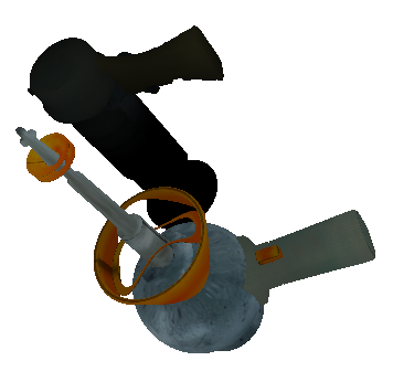
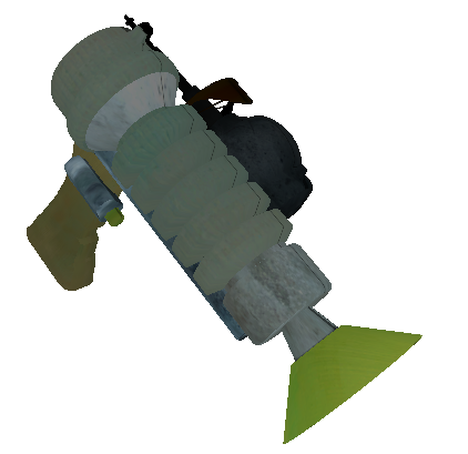
3) Modify the C9_fog demo to implement a simple form of “depth cueing.”
Like Gooch shading, depth cueing is a nonphotorealistic technique that
may help CAD designers when, for instance, viewing complex wireframe models
(although here we’re not using wireframe models). Change the pixel color
calculation to multiply the texColor by the fogFactor, instead of
linearly interpolating between the fogColor and the texColor. Also change
the computation of the fogFactor to follow this linear “depth cue”
formula (instead of
the “fog” exponential formula):
fogFactor = max(0,min(1, (e – fogDistance)/(e-s))),
where e and s representing the starting and ending coordinate of
the depth cueing effect (i.e. anything beyond e is not seen, anything
closer than s looks the same).
Also change fogDistance to be the z coordinate
of eyeposition instead of the length
of the eyeposition vector.
Normally e and s would be passed in from
the main application through variables, but to avoid having to edit
the Setup file to add these variables, you may set e and s in your code.
Experiment with values of e and s for your particular scene to get
a good illustration of the depth cueing effect.
Warning: If I recall correctly, the Cg Tutorial software uses a right-hand
coordinate convention, so e and s may need to be negative numbers.
Use
“Open Scene” to load in an object that’s not the default cityscape model.
Experiment with values of e and s for your particular scene to get the
a good illustration of the depth cueing effect, and take a screenshot.
Here’s a couple of depth cueing examples I threw together. Your mileage will
vary:
4) Load the C8_bump demo. Move the light around (you can select to have
the mouse move the light instead of the scene from the via the Control) menu
and marvel at the drama of the bump mapping effect.
Make a modified version of the bump demo with the following tweaks:
- The fragment shader uses a “normalization cube map” because some
older GPUs didn’t include a normalization instruction (or even floating point)
in their fragment shaders. Since we’re using modern GPUs with a normalization
command, change the code to use “normalize” instead of the normalization
cube map. (Note: This demo is set to compile with a profile appropriate
for older graphics cards. You will need to change the profile on the
fragment shader via the Compile->Configuration menu option and upgrade it
from fp20 to fp30 so your fragment shader will have access to the
normalize function.) Remember, I made a specific reference to this issue near
the end of one of the lectures on shaders.
- Let’s make the scene moodier by incorporating a spotlight effect;
see the “Spotlight Effect” slide in the “Lighting & Rasterization” lecture.
We will
multiply the intensity from dot(normal,light) calculation already given
in the code by this spotlight term. We need to be careful not to be mislead
by the variable names; lightDirection indicates the direction
from the light to an arbitrary point on the surface. For a spotlight, we
need to think of it as pointed in a particular direction; we’ll assume the
spotlight is always pointed at (0,0,0) in object space (which is the
coordinate system this particular example takes place in). Hence, we’ll
need to pass in the raw lightPosition to the fragment shader. You can
do this by outputting from the vertex shader via TEXCOORD2, and hence
inputing it to the fragment shader via TEXCOORD2. (Remember that the vertex
shader will compute this “lightPosition” for three points, and the GPU will
handle the task of linearly interpolating those values across the face of
the polygon when figuring out what pixels to give the pixel (aka fragment)
shader.)
In the spotlight formula in the lecture slides, the vectors must be normalized,
so you’ll need to do another call to normalize. Choose a power sufficiently
high that the spotlight effect is quite dramatic.
Take a screenshot. (You will need to use the default
flat wall; doing bump mapping
on an arbitrary surface is more complex, and not something we
covered in class.)
5) Let’s now play with the C6_particle demo. This is quite different
than others; here, instead of rendering triangles, the API tells the GPU
to plot points at the position indicated by the fragment output
register POSITION that
are squares of size indicated by fragment register PSIZE.
Play with the various parameters in the demo a bit to get a feel for how
it works. Be sure to move the camera around to see the particle fountain
from different angels.
It appears that the input variable “vInitial” is set to random
values, with the range of those random values set by the “Start velocity”
sliders, whereas the “Acceleration” sliders set a constant uniform
“acceleration” variable. The tutorial code generates new particles and
terminates them after a certain amount of time, and increments the time
variable for each particle.
In this problem, we’ll take advantage of the Acceleration sliders to
represent things that aren’t acceleration. We won’t bother to change the
names (that way we can avoid changing the ini file), but be sure to realize
we’re using them for another purpose.
Let’s change the calculation of the particle position to this:
float4 pFinal = pInitial +
           float4(0.1*acceleration.x*t*sin(acceleration.y*t+vInitial.x),
                  0.1*acceleration.x*t*cos(acceleration.y*t+vInitial.x),
                  t*4,0);
How did I come up with this formula? I wanted to simulate a Swirling Cone
of Doom, something kind of like an orderly tornado. This could be a spell
cast from a magic wand, or it could eminate from an alien spacecraft. Note
that the z-position of the particle just marches foward linearly in time.
The other two coordinates spiral outward in a circle. The acceleration.x
variable has been hijacked to control radial velocity, and the
acceleration.y variable has been hijacked to control the speed of the spin.
(Note that the acceleration sliders only do negative numbers; this isn’t a
problem, just realize that to the left is faster and to the right is slower.)
I experimentally set the constants 0.1 and 4 so we’d get reasonable
control ranges without having to change the “inf” file. I’m using vInitial.x to
generate a random starting phase for the spin; by setting Start Velocity X
to its highest value, we get an approximately uniform random starting phase.
Let’s also change the pointSize to be a constant 2, and change the color
scheme to be appropriate for a Swirling Cone of Doom. Let’s have it fade
from some color to white by setting two of the color components to
c*t (it will automatically saturate to 1 when rendering the color) and
setting the other component to 1. This will crossfade from some color to
white. Pick either red, green, or blue to be the color component you set
to 1, depending on which color you think indicates more doom. You will need
to set c experimentally; tweak it until you like the effect.
Play with the “Acceleration X” and “Acceleration Y” sliders, and the camera
position until you get something you think looks really cool. Deselect
Animate Time under the main menu to freeze the animation, and take
a screenshot of your Swirling Cone of Doom.
6) Let’s pull up the simple C3_texture demo; we’ll modify this to wave
in a strange mirage-like fashion.
To add a time element, we will need to tweak the Setup (i.e., the .ini) file
a little bit. You will need to change the SceneType definition to be
“default animateTimeAtStart,” and you will need to add the line
“float time:Time”; below the string definitions.
You’ll also need to add “uniform float time” to the
fragment shader parameter list. (Sorry for all the weirdness;
the method of defining scenarios in the
“ini” file is particular to this Cg Tutorial program, and not something
you’d be likely to see elsewhere.)
Instead of just using texCoord in the texture lookup in the fragment shader,
you should first add a time-varying function of the form
A*sin(B*texCoord.y)*sin(C*time) to the the xcoordinate of texCoord and
D*sin(E*texCoord.x)*sin(F*time) to the ycoordinate of texCoord.
(To get access to the “sin” function, you’ll need to use the
“Compile->Configuration…” menu item, while having the fragment shader tab
selected, to change the fragment profile from
fp20 to fp30.)
Notice
the deformation in x is determined by the y coordinate, and the deformation
in y is determined by the z coodinate. A and D control the amount of
deformation, B and E sort of set the distance
between “deformation valleys”, C and F control the speed. Pick A to be
different than D, B to be different than E, and C to be different than F.
Useful ranges for A and D are roughly on the order of 0.005 to 0.03, B and E
are from 10 to 200, and C and F are 5 to 30.
When you run it, you should see the picture morph in strange oscillatory
ways. Experiment with various values of the parameters. You can also try
using texCoord.x in the deformation formula for the x-coordinate and
texCoord.y in the deformation formula for the y-coordinate. At an
appropriate moment, deactivate “Animate Time” under the control menu
to freeze the animation, and take a screenshot.
<!–
9) Load the C9_projTexturing demo. Play with the camera and light positions;
in particular, zoom the light (use Ctrl-mouse) so that you see many copies
of the texture. You should observe strange effects when many small versions
of the texture appear packed in one space. Take a screenshot.
–>
Not a problem, but an interesting aside: Check out Section 8.4.4
on Valves’ “Half Lambert Diffuse” lighting in this paper on
Shading
in Valve’s Source Engine.
Deliverables: Assemble your Cg code and screenshots in an orderly
fashion into a single Microsoft
Word document or PDF file (using whatever tools you wish to create a PDF).
For each problem above, give the code, then give the screenshot. You only
need to show code for shaders that you modified; i.e. if you had to modify
the vertex shader but not the fragment shader, you need only show the vertex
shader (and vice-versa).
Include “HW3” and as much
as possible of your full name in the
filename, e.g., HW5_Aaron_Lanterman.doc. (The upload
procedure should be reasonably self explanatory once
you log in to T-square.)
Be sure to finish sufficiently in
advance of the deadline that you will
be able to work around any troubles
T-square gives you to successfully
submit before the deadline. If you have
trouble getting T-square to work,
please e-mail your compressed
file to Prof. Lanterman at lanterma@ece.gatech.edu,
with “MPG HW #3” and your full
name in the header line;
please only
use this e-mail submission as a last resort if T-square isn’t working.
Ground rules:
You are welcome to discuss
high-level implementation issues
with your fellow students,
but you should avoid actually looking at
one another student’s
code as whole, and
under no circumstances should you be copying
any portion of another student’s code.
However, asking another student to
focus on a few lines of your code discuss
why a you are getting a particular
kind of error is reasonable.
Basically, these “ground rules” are
intended to prevent a student from
“freeloading” off another student,
even accidentally, since they
won’t get the full yummy nutritional
educational goodness out of the assignment if they do.
Looking at
code from homeworks done in previous years is strictly prohibited.