Colton-Kirsch Inverse Scattering Algorithms

Main	Links	Papers
Research	Project Only	UIUC Only

Inverse scattering algorithms have generally fallen into two broad
categories: fast, approximate linear algorithms
(often based on fast Fourier transforms)
or slow, accurate nonlinear algorithms. The linear algorithms often
amount to simply inverting a Fourier transform. By contrast, nonlinear
algorithms, such as the Distorted Born Iterative Method, usually require
some sort of computationally expensive Newton-like search.
Historically, there have been few options available between these two
extremes.
A notable exception is the so-called “regularized linear sampling” method
developed by David Colton, Andreas Kirsch, and their colleagues.
Although the Colton-Kirsch methods have received much attention
in the mathematical literature, they do not seem to be very well known
in the engineering community. This web page seeks to bridge that gap.

Although some immensely complex mathematical theory underlies Colton and
Kirsh’s method, the resulting algorithm is remarkably simple. In the
original method, for each point
y in the desired image, one solves a linear
equation Fg = f(y) for g, where
f(y) is a vector of complex exponentials
which depends on the position
of the point and F is a matrix formed from the measured data.
The theory dictates that the norm of g becomes large at the border
of the scatterer. Hence, to visualize the scatterer surface, one can simply
plot an image of the norms of the g‘s.
Since the measurements F are typically noisy, the method has been
extended
to incorporate regularization via Morozov’s discrepancy principle.
This principle allows for the fact that the uncertainly lies in the operator
F, instead
of the right hand side f (as is typical in most applications).
We will refer to this method as CK-A (without regularization) or
CK-AR (with regularization).
Note that although the algorithm involves solving sets of linear equations,
it is represents a highly nonlinear kind of processing. It also does not
assume any linearizing approximations (such as the Born or Kirkoff
approximations which underly most linear reconstruction algorithms).

A remarkable aspect of the method is that no a priori knowledge of the
boundary condition is needed.
The exact same perscription holds
for Dirichlet, Neumann, or impedance boundary conditions. This is in
sharp contrast to traditional iterative nonlinear methods, which require
prior knowledge of the boundary conditions. It is also helpful in cases
where the scatterer is a penetrable, inhomogenious medium; in these
situations, the method gives the support of the scatterer. The method has
hence been helpful in biomedical applications, such as
detecting leukemia.

Kirsch
derived a variation on the method which involves solving
(F^star F)^{1/4} g = f(y) (please forgive the pseudo-Latex)
at each point,
and again looking for points where ||g|| blows up.
We will refer
to this method as CK-B (without regularization) or CK-BR
(with regularization).

Most of the work on Colton-Kirsch methods has been in two dimensions.
The scatterer is assumed to be an infinitely long cylinder whose profile
does not change along the z-dimension. In the acoustic case, one can
then deal with 2-D Helmholz equation. In the electromagnetic case,
if the field is polarized so that the electric or magnetic fields runs
parallel to the axis of the scatter, Maxwell’s equations reduce to the
2-D Helmholz equation.
Although the method has been extended to the three-dimensional scalar case,
our exposition will focus on two dimensional problems.

Simulated Data

We simulated scattering data for these airplane shapes:

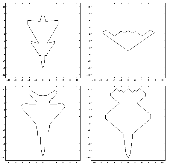
The shapes are top-down
profiles of the VFY-218 (upper left),
the B-2 (upper right), the F-15 (lower left),
and the YF-23 (lower right).
Remember that we
are assuming the objects are infinitely long cylinders,
and not the three-dimensional shape of the original aircraft.
The VFY-218, F-15, and YF-23 are is approximately 15.5, 19.5, and 20.5
meters long, respectively. Although the real
B-2 is much larger than the other aircraft, we have artifically scaled
our model to make it 15.5 meters wide.
We computed data at 100 MHz and 200 MHz for both TE
and TM polarizations,
with c = 3 times 10E8 meters per second. A full 360-degrees of
incident and observation angles were used, with data computed at three degree
increments, so F is a 120 by 120 matrix.

Reconstruction Results

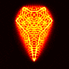
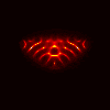
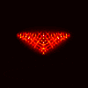
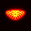
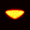
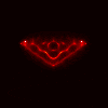
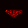
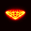
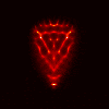
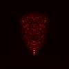
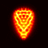
The images in this section are 100 by 100 pixels, with a spacing of
0.25 meters between pixels. We show reconstruction results using the
CK-AR and CK-BR methods. (We use the regularized methods even though we
have not explicitly added any noise to the data.)

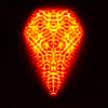
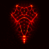
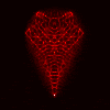
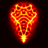
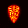
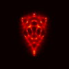
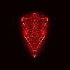
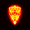
We are displaying 1/||g|| (the reciprocal of the norm of g) on
a heated object scale. Hence, large ||g||,
which we expect approaching the
boundary, are indicated by black. Small ||g|| are indicated by
bright colors like yellow and white. (Interestingly, the outline of
the scatter is most clear where we see yellow – i.e. where ||g||
is small! We currently do not have a good theoretical explanation as to why.)

Some of
the CK-AR images look a bit dim, since a couple of pixels usually are
of much greater magnitude than the rest – this could be remedied by
adjusting the color scale, but we haven’t done that here.

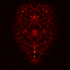
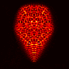
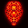
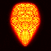
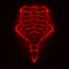
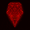
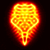
Here are the results for the YF-23.
Top row corresponds to the TE case, bottom row to the TM case.
From left to right, the columns correspond to: CK-AR at 100 MHz,
CK-AR at 200 Mhz, CK-BR at 100 MHz, and CK-BR at 200 MHz. (Notice that
the TM case results in much clearer reconstructions than the TE case.)

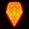
Here’s the results in the same sequence for the F-15:

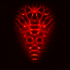
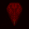
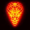
Here’s the results in the same sequence for the scaled B-2:

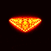
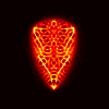
Finally, here’s the results in the same sequence for the VFY-218:

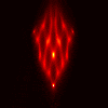
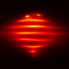
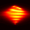
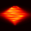
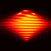
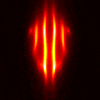
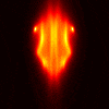
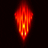
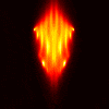
Limited Angle Experiments

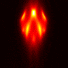
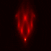
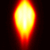
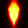
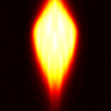
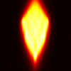
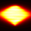
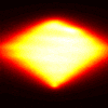
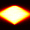
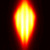
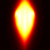
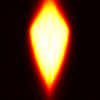
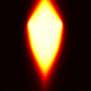
Here are some experiments using the VFY-218 shape
in which we tried using a limited aperture.
The incident and observation apertures are coincident and of size
60 degrees (so one is essentially using 20 by 20 submatrices of
F). The following images use CK-AR. The top, middle, and bottom
rows correspond to illuminations/observations from the bottom, side, and
top, respectively. From left to right, the columns correspond to:
TE case, 100 MHz; TM case, 100 Mhz, TE case, 200 MHz, TM case, 200 Mhz.

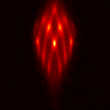
These images are as above, except using CK-BR:

---

Last updated 8/17/00. Send comments or questions to
lanterma@ifp.uiuc.edu.